
#2: Understanding Numerical Errors For Physics Simulations
Finally learn the secret to more accurate simulations!

Hey, Nasser here!
Hope you had a great week and are fired up for this edition of Compute This!
In today’s post:
Solver setup is important.
Types of numerical error.
How to reduce the errors and get more accurate results.
[Download] Python code to practically explore numerical error.
Consider supporting my work
Let’s get into it!
1. Solver setup is important
Setting up a new simulation study is an involved process.
100’s of options, settings, pre-processing steps and preparation can leave you in a state of confusion and overwhelm.
Some of the most important parameters to get right revolve around the solver settings.
The following is a typical setup requirement. Note the options surrounded by the yellow box.
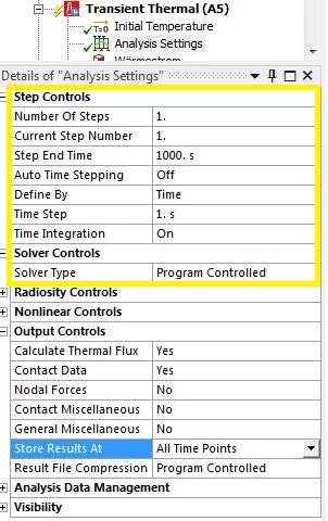
Getting these ‘right’ involves understanding how a solver works as well the time you have, compute resources etc.
These settings directly correspond to the accuracy of the results.
2. Types of numerical error
After setting up the solver, you hit the ‘Solve’ or ‘Start’ button and set off chain of events.
Numerical equations are being solved for each and every ‘time step’ it takes forward.
Let’s go further and consider a ball flying through the air (aka projectile).
It has an initial position
It has an initial velocity
Gravity is enabled
Let’s say 100 time steps are to be taken forward in time.
This means at each time step the solver will need to calculate the position of the ball by solving the equations of momentum - acceleration and velocity to give position.
Let’s watch this in action:

There are two types of numerical error present in every numerical simulation:
Local - errors that occur within a single time step.
Global - errors that accumulate from time step to time step.
3. How to reduce the errors and get more accurate results
Error control depends on the integration scheme used in the solver - this is the method used to approximate the solution to the numerical equations in each time step. ‘Euler’ and ‘RK4’ are examples of integration schemes.
The errors produced by both schemes compared against the accurate analytical solution:
RK4 is considerably more accurate and remains so over the duration of time steps.
For local errors it’s possible to use a smaller time step. The trade-off is that the simulation time will increase, often by a significant amount.
Global errors remain controlled with better integration schemes like RK4 since it considers intermediate calculations per time step. However, this will usually make it slower, albeit more accurate.
4. Download the Python script!
Download the Python script below, changing the time step value (‘dt’ around line 8) and running the code again within Jupyter Notebook (nothing to install!)
Understand and control numerical errors better than the Engineer / Researcher next to you.
Instructions:
Download the file above and rename it with a .zip file extension
Extract the text (.txt) file from the zip
Copy the complete Python code and paste it into Jupyter Notebook (the online Python code editor)
Click on the Play button in the toolbar (‘Run this cell and advance’) as highlighted
Edit the time step (‘dt’) and re-run to see the differences in error.


Thank you for reading and I hope you found it valuable this week.
Share Compute This! with others and get a FREE shout-out, mention or your website (personal or business) link advertised on a future issue!
Comment and provide feedback to suggest future content.
Until next time, have a great week ahead!
Nasser