
#1: How I Simulated 2D Heat Transfer In An Excel Spreadsheet!
Step-by-step - nifty, gritty details inside with an exclusive download!

In this weeks issue:
The LinkedIn post that started this Newsletter
Explaining Heat Transfer
Why Excel is a great playground for physics simulations
Step-by-Step implementation + results video
Updated Excel file download (v2)
Hello fellow Computes!
Welcome to the very first edition of Compute This!
Last week I posted the results of a simulation I created in Excel and my LinkedIn inbox was on fire…

100+ reactions, 15+ file requests and 90+ new followers in a little over 48 hours.
Insane for someone that didn’t expect too much to result from a 30 minute experiment!
So what’s the big deal?
Heat transfer is a natural, real-life phenomena.

Thermal energy is transferred through between physical objects
Heat will tend to move from high to low temperature regions
There are 3 types: conduction (solids), convection (liquid & gases) and radiation (all) [2]
Engineers and Scientists developing new technologies or products need to be acutely aware of thermal performance with respect to cooling and safety.
However, most Engineers and Scientists use Excel to capture and record raw experimental data, not to carry out simulations.
I decided to do just that!
Why? Because Excel is actually a great ‘canvas’ to explore problems like numerical calculations over a series of time steps.
Through the eyes of a software programmer, Excel is nothing more than a program made of logic, a GUI and built-in maths libraries. Consider:
The spreadsheet is a grid of cells (numerical solvers require the ‘domain’ or geometry of interest to be made into smaller parts (aka discretised) for calculation.
You can enter formulas into each cell and add relations to adjacent cells (perfect for neighbour checks and updates).
Excel is programmed to update every formula in a sheet and has a ‘Solver’ function that allows you to set the iteration counts).
Excel exposes a VBA programming interface that allows users to write custom scripts (used for custom controls in this particular case).
Step-by-step setup
Using the knowledge above, we can formulate a numerical simulation as follows.
Initialise a grid of 10x10 size. The outer cells are our ‘boundary’ conditions, we later set to 0 and the central four cells set to a value of 100.
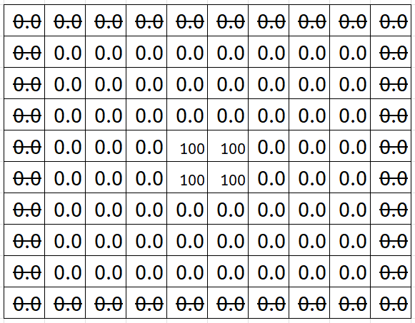
Set some ‘conditional’ formatting to colour the cells based on value. To do this, go to Home > Styles > Conditional Formatting > Styles and set the minimum to blue and maximum to red for a traditional simulation heat colour scale. You should now have something that looks like the following image.

Heat transfer can be modelled by using the equivalent numerical approximation for the ‘Fourier’s Law’. You will need to do this for each inner cell, considering the neighbouring 4 cells. Doing this for cell C3 will give you:
\(=C3 + alpha * dt / dx^2 * ((B3 + D3 + C2 + C4) - 4 * C3)\)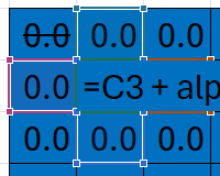
Copy the formula to all of the inner grid cells, leaving the boundary cells set to 0. Ensure the central 4 cells are set to 100 if overwritten. This will be our initial value condition.
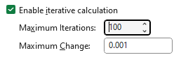
Set the solver settings to 100 steps / iterations. Go to File > Options > Formulas > Enable Iterative Calculations
Press F9 to solve the formulas for each cell over each step.

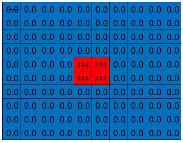


Here are the results:
I added graphs to collect and plot values from across the symmetric center, giving you a plot of temperature, updated with each time step in real-time.
Updated simulation
New native ‘Simulation’ control bar with custom macros
Buttons to reset the grid and step through simulation updates automatically
Option to select 2 cases → heat from center vs heat from one side
User-friendly, easy to use
All contained within Excel!
NOTE: Upon downloading the file below, be sure to rename the extension from .cbz to .zip in order to extract and run the Excel file on your computer. I had to rename the file to upload here as the newsletter platform does not support .zip files directly. Thanks.
Fellow Computes, please consider supporting my work if it has helped you in any way 🙏
I personally create, run and manage this newsletter. I take the time to bring you valuable content, manually curated and developed to inspire, educate and inform readers like you.
To help me keep this newsletter free, with high-quality valuable content consider supporting my efforts directly:
The take-away
You can do numerical analysis using a calculator, spreadsheet software like Excel or by writing your own programs altogether in a programming language.
Numerical approximation is a mathematical technique that solves for unknown values, all it takes is for you to convert fundamental laws into numerical approximations.
I sincerely hope you enjoyed this edition. I’m always looking for good content ideas, so feel free to suggest what you’d like me to look at / experiment.
Until next time, keep computing my fellow Computes!
-Nasser 👋
References:
[1] https://termopasty.com/en/thermal-conduction/
[2] https://www.greenspec.co.uk/building-design/heat-transfer-conduction-convection-radiation/
Disclaimer:
The content in this newsletter is for educational purposes only curated and / or developed by me. It does not reflect the views, opinions or capabilities of any employer, sponsors, referrers or associates.
This is awesome. Can you help me create one for a cylinder? With unsteady heat conduction calculations based on different materials?
What did you like most about the results? Did you like this post? Leave me some comments, I always read all of them.