
The Finite Volume Method (FVM) - a visual guide!
And a peek into how OpenFOAM does it!


I’m a very visual guy with it comes to learning - especially abstract concepts.
In fact, whilst I can understand complex topics (if I slow down), I’ll insist on sketching EVERYTHING out.
It wasn’t always like this.
I realised when I was struggling at School, College and even when I started out at University.
I was met with a bigger adversary - Engineering mathematics.
I had to do something more than just try and "absorb” the black and white text in front of me.
Instead of blaming the Lecturer’s for not explaining it well (this was true on occasion), I considered my own study techniques.
This made all the difference and I’ll take you through it to explain the Finite Volume Method (FVM) - the numerical methods used by OpenFOAM!
Let’s get to it…
1. What are we really solving for?
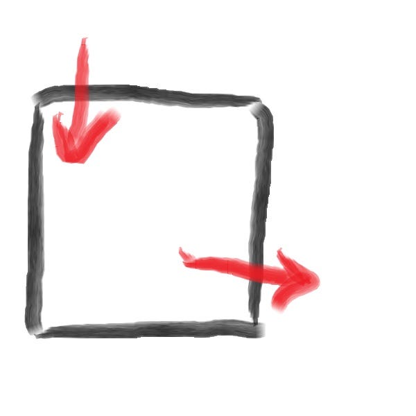
Consider a box like the one above.
In FVM terms, the box is called a “control volume” (aka the domain).
And we’re solving the law of “conservation”…
Change inside the box = what comes in – what goes out + sources inside.
Whether that’s heat, fluid or any other energy source (marked by the red arrows).
Energy and matter doesn’t disappear - it all goes somewhere.
(High-school maths 101, I know…)
But principles like this are better visualised in my opinion.
2. Control Volume and a Mesh
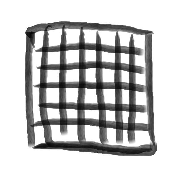
The Mesh “discretises” or reduces the space we are interested in into smaller parts.
Each cell of the mesh needs to check it’s neighbours to calculate the differences in heat, density etc. between them. For example, the current cell being checked (in blue) has 8 neighbours (in green) in this 2D case:
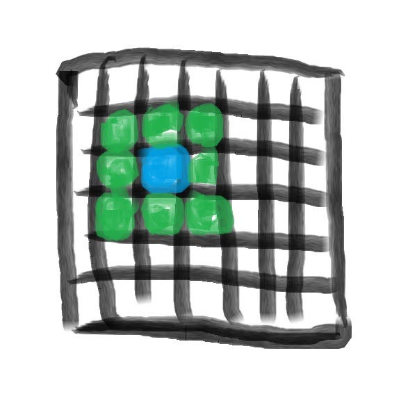
This process of iterative, step-by-step calculation and update makes this algorithm perfect for Computers!
Repeatable and scalable…
3. Adding time into the equation
We have the space, now we use the concept of Time in our calculations of the changes our field properties.
This is done inside the numerical equations used in FVM algorithms.


In the example above, from left to right, we can see our domain at time t (before) and t+1 (after).
At each time step the Computer updates the value in every cell based on its neighbours. Over many time steps, this simulates how heat or fluid evolves throughout the domain.
4. the OpenFOAM Connection
OpenFOAM is not a black-box, it’s open-source but can be daunting to look at in all of its raw form (code).
You may have used the fvSchemes file in a simulation setup.
Well, within here we define the numerical scheme to use. For example:
An “Upwind” fvScheme refers to values being used in upstream cells
A “Central” fvScheme refers to using the average of two neighbouring cells
A closer look at the code from a simple OpenFOAM solver reveals this the general solver step:
fvm::ddt(phi) + fvm::div(phi*U) - fvm::laplacian(D, phi) == SuAnd that wraps up FVM!
A few parting words
Whilst it’s been around for some time, the FVM method is fascinatingly simple in principle. I avoided heavy mathematical notation and formulas here on purpose.
Remember, each cell / box of a Mesh solves one equation and together they form a system being solved, one step at a time.
Brilliantly simple, very effective and actually quite accurate.
Thank you for reading - help me spread simulation clarity further, like and share if you found it helpful!
Until next week. 👋
Nasser
When you're ready, I can help you in other ways…
🎓 Learn about CFD, simulation and digital engineering from me daily.
Follow me on LinkedIn: https://www.linkedin.com/in/nassermushtaq/
📢 Advertise your engineering educational product or open-source tools to my fast-growing audience. I write here to 500+ subscribers and also more frequently on LinkedIn to 4500+ followers. Email me directly at: hi@nasserm.com
Disclaimer:
All content in this post and newsletter is my own production and do not reflect the opinions or positions of my employers, partners or associates.